Uncategorized

The (lack of) relation between youth playing time and later success in football

Picture the scene: You’re a football manager. You’re in charge of a big club with a good youth academy, and you want your academy players to succeed. Good prospects need playing time… but you’re chasing the Champions League positions, and you can’t guarantee a starting slot for your promising but unproven 19 year old. You could loan him out to a smaller team so he gets game time… but good prospects also need to learn from watching the best at work, and your 19 year old won’t pick up the highest level tips and tricks on a League One training ground.

It’s a dilemma. Do you loan him out for game experience and deprive him of the chance to study with the best, or do you keep him around the squad for the learning opportunities and deprive him of the chance to learn how to adapt to match situations?

As a Charlton Athletic fan, my instinct is to say loan him out. Despite Duchatelet’s concerted efforts to completely ruin us, we’ve got one of the best academies in the country, and the big clubs are often hovering around, ready to swoop. I certainly can’t begrudge our players moving on to bigger and better things, but it seems that our players stall once they get to big clubs and stop playing so much. Jonjo Shelvey, for example; he was running our midfield in League One, but it felt like he went backwards once he got to Liverpool and spent all his time on the bench. Surely, many of us felt, it would be better for Liverpool to have loaned him straight back to Charlton; we’d have had an excellent player getting us into the Championship, and they’d have had a player gaining valuable match experience.

This is all just post-match pub conjecture, but luckily, there’s the internet, which is basically an all-you-can-eat buffet of sports numbers. So I’ve been mining the Charlton Athletic youth team page on transfermarkt to extract playing data for all our academy footballers over the years.

Writing the code for this took many, many hours. Unlike cricinfo, the site isn’t configured in a very scrape-friendly way… but hey, it was an amazing regex workout. I’ll post a 700-odd line script another time.

Once you’ve got a lot of data, you can do all kinds of stuff with it. The difficult thing is asking the right questions.

What I want to know is whether more playing time as a young player is related to greater success later on. Measuring “success” as a footballer is a very vague notion, so let’s refine it a bit:

Does playing more games at any level when under 21 mean playing more games at the top level when over 21?

I’m going to arbitrarily define “top level” here as the English Premiership, Spanish La Liga, Italian Serie A, German Bundesliga, French Ligue 1, as well as Champions League and UEFA Cup / Europa League matches. Feel free to argue with me in the comments!

This is a lot easier to work out. We also have to refine it to looking at players who are already over 21 so that we’ve got post-21 career success to look at. This means not including players like Joe Gomez because he’s still only 19, so his 31 under-21 appearances and 0 over-21 appearances will through the data. I’ve limited it to players who are currently older than 24, with the opportunity for at least three full seasons aged post-21. Also, this analysis does not include goalkeepers, as the higher competition for places means that many second-choice goalkeepers never play at all.

Right, so let’s look at my intuition:

CAFC annotated game appearances graph

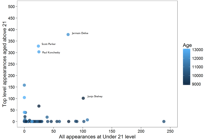
…my intuition isn’t very good. There’s no relationship between how many games a player features in and how many top level games that player features in (r = 0.05, p = 0.74).

(Age on the graph is expressed in days, by the way. Leap years make time calculations hugely frustrating.)

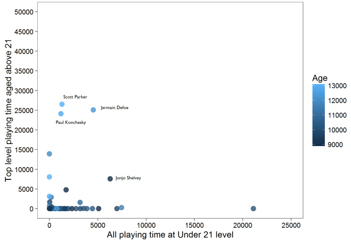
It could be that these correlations are thrown off by lots of late substitute appearances; you technically count as making an appearance regardless of whether you play the entire game or come on at 89 minutes to run down the clock.

So, I repeated it for actual number of minutes played… and it’s the same kind of picture (r = 0.0, p = 0.99):

CAFC annotated game time graph

It looks like my feeling about youth game experience being related to future success is inaccurate. But, this is pretty small data, taken from one club’s youth team players. It could be different if we use more teams. It’s also pretty relevant that Charlton aren’t actually very good; you might be getting regular game time at 20 years old in the Championship, but that may well be your level.

So I also had a look at Premiership youth team players at big clubs. I took the teams which have been in the Premiership the whole time (thus excluding recently successful teams like Manchester City) and relatively consistent performers – Arsenal, Manchester United, Chelsea, Liverpool, and Tottenham Hotspur. Whereas Charlton can give promising youth team players like Ademola Lookman a decent run (get your hands off him, please, we’ve got to escape League One again), it’s more of a risk for these larger teams to play untested potential over proven performers. The dilemma outlined at the start is more pressing for the big teams, so they (presumably) have more of a vested interest in solving it.

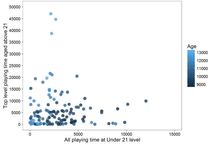
So is there a relationship between under-21 appearances at all levels and career success as measured by post-21 top level appearances?

big teams game apperances graph

…no. This time I’ve excluded players with zero appearances on either of the two axes because it was messy, and because there’s enough data points to look at players with both. There’s still no correlation at all (r = -0.06, p = 0.48).

Again, the same goes for actual playing time (r = -0.03, p = 0.72).

big teams game time graph

This still feels counterintuitive to me, but the data is clear: there’s no relation between game time as a player under 21 and later career success, whether you started at a poor Championship team like Charlton or a consistent big Premiership team.

This doesn’t mean that sending players out on loan to smaller clubs is actively bad for their development. Nor does it mean that keeping young players in the squad at the expense of playing time is better for their development. Rather, what it shows is that developing a young player is dependent on all kinds of factors, and that simple game time is no predictor of later success. When deciding whether to send a young player out on loan or keep him around the squad, club and academy managers should keep in mind that there’s no general tendency for either decision to be the correct one, and what’s best for one player will probably be completely different from what’s best for another.

Standard
Uncategorized

Quiz time: La Liga or Premier League?

Last week, I wrote about visualising league tables spatially to reflect the points differences between teams. Inspired by Stephan’s tweet on comparing violin plots of points-per-game distribution across the big five leagues, I thought I’d address something that’s been irritating me for a while.

If you’re in the UK and start talking to somebody about European football, chances are they’ll say something a little like this:

“Right, yeah, English teams are bobbins in the Champions League because the Premier League might not have the highest quality, but it’s the best league in the world because of the competition and how close all the teams are. You never know who’s going to win it! It’s not like in Spain, where it’s always going to be Barcelona or Real Madrid winning it by a mile, and all the other teams don’t even matter.”

According to this stereotype, a spatial dotplot of the Premier League would look like this:

premier league stereotype

…while a spatial dotplot of La Liga would look like this:

la liga stereotype

This is a stereotype which may or may not be true. So, I’ve taken the tables from the Premier League and La Liga for the last ten completed seasons (2005-06 through 2014-15), and plotted the dotplots for each season with the two leagues side-by-side.

That was pretty useful, but then I figured, hey, I’m a cognitive neuroscientist, I spend most of my time experimenting on people… why not try that with football fans rather than bored undergraduates?

So here’s a quiz!

You will see dotplots of the two leagues side-by-side for a given season. All you have to do is guess which league is on the left and which league is on the right.

If La Liga and the Premier League conform to the (British) stereotype, it should be easy enough to guess which league is which from looking at the dotplots. In that case, the average score will be something like seven or eight out of ten. If not, it’ll be harder to guess which is which, and the average score will be fairly close to chance, probably somewhere between four and six out of ten.

Please have a go – it only takes about two minutes (if it takes longer than that, I know you’re cheating by looking it up!) – and share it with anybody who’s interested. The more people do it, the more accurate an average result there will be.

Here’s the full link – no registration or anything else needed:

https://www.qzzr.com/c/quiz/199280/english-premier-league-or-spanish-la-liga

I’ll write a follow-up blog with the full tables and details and results in a couple of weeks.

Standard
R, Uncategorized

Visualising football league tables

I was looking at the Premiership league table today, and it looks like this:

current league table

It’s pretty informative; we can see that Leicester are top, Aston Villa are bottom, and that the rest of the teams are somewhere in between. If we look at the points column on the far right, we can also see how close things are; Villa are stranded at the bottom and definitely going down, Leicester are five points clear, and there’s a close battle for the final Champions League spot between Manchester City, West Ham, and Manchester United, who are only separated by a single point.

Thing is, that requires reading the points column closely. If you take the league table as a simple visual guide, it doesn’t show the distribution of teams throughout the league very well. If you say that Stoke are 8th, that sounds like a solid mid-table season… but what it doesn’t tell you is that Stoke are as close to 4th place and the Champions League as they are to 10th place, which is also solid mid-table. A more visually honest league table would look something a little like this*:

current league table dragged about a bit

*definitely not to scale.

Screen-shotting a webpage and dragging things about in MS Paint isn’t the best way to go about this, so I’ve scraped the data and had a look at plotting it in R instead.

Firstly, let’s plot each team as a coloured dot, equally spaced apart in the way that the league table shows them:

League position right now

(colour-coding here is automatic; I tried giving each point the team home shirt colours, but just ended up with loads of red, blue, and white dots, which was actually a lot worse)

Now, let’s compare that with the distribution of points to show how the league positions are distributed. Here, I’ve jittered them slightly so that teams with equal points (West Ham and Manchester United in 5th and 6th, Everton and Bournemouth in 12th and 13th) don’t overlap:

League points right now

This is far more informative. It shows just how doomed Aston Villa are, and shows that there’s barely any difference between 10th and 15th. It also shows that the fight for survival is between Norwich, Sunderland, and Newcastle, who are all placed closely together.

Since the information is out there, it’d also be interesting to see how this applies to league position over time. Sadly, Premiership matches aren’t all played at 3pm on Saturday anymore, they’re staggered over several days. This means that the league table will change every couple of days, which is far too much to plot over most of a season. So, I wrote a webscraper to get the league tables every Monday between the start of the season and now, which roughly corresponds to a full round of matches.

Let’s start with looking at league position:

League position over time

This looks more like a nightmare tube map than an informative league table, but there are a few things we can pick out. Obviously, there’s how useless Aston Villa have been, rooted to the bottom since the end of October. We can also see the steady rise of Tottenham, in a dashing shade of lavender, working their way up from 8th in the middle of October to 2nd now. Chelsea’s recovery from flirting with relegation in December to being secure in mid-table now is fairly clear, while we can also see how Crystal Palace have done the reverse, plummeting from 5th at the end of the year to 16th now.

An alternative way of visualising how well teams do over time is by plotting their total number of points over time:

League points over time

This is visually more satisfying than looking at league position over time, as we can see how the clusters of teams in similar positions have formed. Aston Villa have been bottom since October, but they were at least relatively close to Sunderland even at the end of December. Since then, though, the gap between bottom and 19th as opened up to nine points. We can also see how Leicester and Arsenal were neck and neck in first and second for most of the season, but the moment when Leicester really roared ahead was in mid-February. Finally, the relegation fight again looks like it’s a competition between Norwich, Sunderland, and Newcastle for 17th; despite Crystal Palace’s slump, the difference between 16th and 17th is one of the biggest differences between consecutive positions in the league. This is because Norwich, Sunderland, and Newcastle haven’t won many points recently, whereas Swansea and Bournemouth, who were 16th and 15th and also close to the relegation zone back in February, have both had winning streaks in the last month.

One of the drawbacks with plotting points over time is that, for most of the early part of the season, teams are so close together that you can’t really see the clusters and trends.

So, we can also calculate a ratio of how many points a team has compared to the top and bottom team at any given week. To do this, I calculated the points difference between top and bottom teams each week, and then calculated every team’s points as a proportion of where they are.

For example, right now, Leicester have 66 points and Aston Villa have 16. That’s a nice round difference of 50 points across the whole league. Let’s express that points difference on a scale of 0 to 1, where Aston Villa are at one extreme end at 0 and Leicester are at the other extreme end at 1.

Tottenham, in 2nd, have 61 points, or five points fewer than Leicester and 45 points more than Aston Villa. This means that, proportionally, they’re 90% along the points difference spectrum. This means they get a relative position of 0.9, as shown below:

Relative league position over time

This is a lot more complicated, and perhaps needlessly so. It reminds me more of stock market data than a football league table. I plotted it this way to be able to show how close or far teams were from each other in the early parts of the season, but even then, the lines are messy and all over the place until about the start of October, when the main trends start to show. One thing that means is that however badly your team are doing in terms of points and position, there’s little use in sacking a manager before about November; there’s not enough data, and teams are too close together, to show whether it’s a minor blip or a terminal decline. Of course, if your team are doing badly in terms of points and position and playing like they’ve never seen a football before, then there’s a definite problem.

To make it really fancy/silly (delete as appropriate), I’ve plotted form guides of relative league position over time. Instead of joining each individual dot each week as above, it smooths over data points to create an average trajectory. At this point, labelling the relative position is meaningless as it isn’t designed to be read off precisely, but instead provides an overall guide to how well teams are doing:

Relative league position over time smooth narrative (span 0.5)

Here, the narratives of each team’s season are more obvious. Aston Villa started out okay, but sank like a stone after a couple of months. Sunderland were fairly awful for a fairly long time, but the upswing started with Sam Allardyce’s appointment in October and they’ve done well to haul themselves up and into contention for 17th. Arsenal had a poor start to the season, then shot up, rapidly to first near the end of the year, but then they did an Arsenal and got progressively worse from about January onwards. Still, their nosedive isn’t as bad as Manchester City’s; after being top for the first couple of months, they’ve drifted further and further down. It’s more pronounced since Pep Guardiola was announced as their next manager in February, but they were quietly in decline for a while before that anyway. Finally, looking at Chelsea’s narrative line is interesting. While they’ve improved since Guus Hiddink took over, their league position improvement is far more to do with other teams declining over the last couple of months. Four teams (Crystal Palace, Everton, Watford, and West Brom) have crossed Chelsea’s narrative line since February.

I don’t expect these graphs to catch on instead of league tables, but I definitely find them useful for visualising how well teams are doing in comparison to each other, rather than just looking at their position.

Standard
Education, Open Data, R

The gender gap in school achievement: exploring UK GCSE data

I was reading this article in the Washington Post a couple of days ago. It’s about data from Florida which shows that girls outperform boys at school, and that the gender gap is bigger at worse schools.

It’s well established that girls outperform boys at school, but seeing it visualised and quantified like that was fascinating, and I wanted to reproduce that data for UK schools. We frequently use American statistics to talk about social issues in the UK, which frustrates me; sometimes we’re close enough for it to generalise, but sometimes it doesn’t and it’s like there’s a gigantic metaphorical ocean between the two societies. We know that British girls outperform British boys, but I wanted to see how similar the situation is.

Luckily, the UK government has one of the best records for open data in the world, and so this information is pretty easily found here and here. The main challenge is actually getting through all the data to find the good bits, as so much of it is available, but I found it in the end. So, I shoved all that into R and messed about with some dataframes. Note that I’m not working with private schools here, just state schools… all 2488 of them which have full data for all metrics reported below. Also, all the data is only fully available for England, not the whole of the UK.

The first thing is to decide how to measure achievement. Here, I’m focusing on GCSEs, the standard qualification which most UK teenagers take at 16 and which marks the end of mandatory education. There are two good metrics for measuring GCSE achievement: the percentage of students who get at least five A*-C grades, and the average capped GCSE point score. The first is simple. Students generally take GCSEs in somewhere between seven and ten different subjects, and the percentage of them who score a grade C or above in at least five GCSEs is one of the main metrics that British people obsess over (for people outside the UK, I’m serious, the national newspapers print this figure for all state schools every August when exam results come out). The second is a little more complicated, and it’s explained here. It’s measured by attributing a certain number of points per exam grade (58 for an A*, 52 for an A, and so on down in sixes). It then measures only a student’s top eight GCSEs. So, if you took 11 GCSEs, scored 6 A*s, 4 As, and a B, you’d get 6 x 58 plus 2 x 52 equals 452. This is then averaged across the school. Literally nobody outside government departments ever uses this, but it’s actually a pretty good measure; focusing on the five A*-C rate is a bit blind to quality over quantity, as a student who gets four A*s and four Ds harms the school’s statistics while a student who gets five Cs and three Fs is good for the school’s statistics, despite the first student clearly doing better overall.

The next thing is to decode the wording of the original article: “the gender gap is bigger at worse schools”. There are several ways of talking about what makes a school good or bad, so I’ll focus on three different metrics:

  1. The rating given to each school by the assessment organisation Ofsted. Each school is inspected every couple of years, and gets given an overall grade: outstanding, good, requires improvement, or inadequate. This is a useful, state-sanctioned measure of how good a school is.
  2. The average GCSE achievement data per school. Presumably, better schools get better results. This is a useful measure of how good a school is in terms of what many parents say they care about.
  3. The average wealth of the student body at the school. Let’s face it, when a lot of middle-class British people say “we were lucky enough that our son got into a good local school”, what they actually mean is “we’re so glad there’s no poor people there”. We can measure the average wealth of the student body by looking at the percentage of students who are eligible for free school meals. The higher the percentage, the poorer the student intake.

Firstly, let’s look at the gender gap in GCSE achievement by Ofsted data. This is categorical, so we can have some nice straightforward histograms. Boys are in light blue, girls are in dark pink. Sure, it’s gendered, but it’s an effective and intuitive colour scheme.

histogram of five A star to C rate and each sex per ofsted rating.png

As you’d expect, the outstanding schools get better results than the good schools, and so on and so on. But, it seems that girls outperform boys across the board, regardless of how good the school is (I did an ANOVA on this; the gender gap effect is slightly less for outstanding schools, but it’s a negligible difference. The gender gap at outstanding schools is 7.5 percentage points versus about 8.5-9.5 percentage points for the other three assessments).

histogram of GCSE capped points score and each sex per ofsted rating.png

…and this is mirrored in the capped GCSE points average. Again there’s a tiny bit less of a gender gap in the outstanding schools compared to the rest, but girls do better than boys everywhere.

Right, so much for Ofsted. Let’s look at overall school GCSE achievement. This is continuous, so it’s going in a scatter plot. Plotting every single school’s boys’ and girl’s result was really messy, so this averages across schools on each percentage point on the x-axis (i.e. what you see at 50% is the average boys’ five A*-C rate and the average girls’ A*-C rate across all schools which got a 50% overall five A*-C rate). Likewise in the second plot with every single capped GCSE average points score, where each points score on the x-axis is rounded to a whole number and averaged with others of the same number. Rest assured that the lines of best fit are essentially identical in the larger, messier plots. I did do plots with standard errors, but thought I’d forgotten… then I looked closely, and realised that the standard errors were so small that they were barely distinguishable from the lines.

scatterplot of GCSE results for each sex across GCSE results.png

scatterplot of capped GCSE results for each sex across rounded school capped GCSE results.png

This one tells a clear story, and is very, very similar to Figure 1 in the Washington Post article which shows the standardised maths and reading assessment plot. However, there are two main differences:

  1. If anything the very worst schools seem to have less of a gender gap, especially in the five A*-C rate plot … although this is probably more about a lack of data at that end. (this is one of the few times I think it’s a good thing to have a lack of data)
  2. It basically doesn’t matter how good or bad the school is, the difference between boys and girls is consistent across all levels of achievement. The only place where boys and girls are almost equal is right at the top, where there’s a ceiling effect; assuming that each school is 50% boys, 50% girls, there can’t be a big difference between the two if a school is getting 99% five A*-Cs overall.

And now for the free school meals data, or the middle-class poverty aversion question. I’m going to bombard you with graphs here. First, just to show you, here are the messy ones where all rates for all schools are plotted:


…but like I said, it’s messy and hard to focus on, it’s like somebody spilt muisjes on the screen.

So, here’s the same plots but with all schools averaged together at each data point. This isn’t even at each percentage point, it’s to the nearest 0.1 of a percentage point, because there’s that much data.

scatterplot of GCSE results for each sex acrossfree school meal eligibility rate (loess se).png

scatterplot of average capped GCSE results for each sex across free school meal eligibility rate (loess se).png

This also tells a very clear story. The schools with richer students get better results. I also found out the Pope’s religion, and something about bears and woods. But, again, there are the same two main points:

  1. There seems to be less of a gender difference in achievement at worse (well, poorer) schools, but this is probably because there aren’t that many seriously deprived areas. Not to say we don’t have deprivation in the UK, we definitely do, and it’s growing, but there are very few schools where over half the students qualify for free school meals (which probably says more about our ridiculously strict benefits threshold rather than the state of poverty).
  2. The performance and achievement gap remains even at the very best (well, richest) schools.

There’s also race data available, but I feel like that’s a topic for another blog at another time. This one is already long enough!

The point is this: while the Washington Post article was fascinating, it doesn’t fully generalise to British society. In the UK, the gender gap for school achievement barely gets bigger at “worse” schools, regardless of how you measure what a bad school is… which is a good thing, I guess? In fact, the gender gap for school achievement seems to be entrenched across education achievement and wealth.

Are girls outperforming boys, or are boys lagging behind? Is it both? I’m not an education specialist, I’m just a guy with Rstudio, so I’m reluctant to speculate… but I will anyway.

I think what I’ve ruled out here is any obvious overriding education level or socio-economic effects of the gender achievement gap. It could be that girls are simply more intelligent than boys, although such a simplistic solution seems unlikely. It could be a social peer pressure effect, in that it is more acceptable to be feminine and work hard at school than it is to be masculine and work hard at school (although that wouldn’t explain the reports that this gender difference is present at very, very early ages). It could be that teaching is a female-dominated profession; female teachers may knowingly or unknowingly choose course materials preferred by girls over materials preferred by boys, female teachers may knowingly or unknowingly favour, reward, and encourage problem-solving strategies preferred by girls over strategies preferred by boys, etc. etc., and that this may get entrenched over time. It could be that a culture which encourages and promotes girls’ education, given their denial of access to it until relatively recently, accidentally creates a culture where boys feel undervalued and demotivated. It could be that girls collaborate with each other on homework and exam revision more than boys do, which has been shown to effectively improve learning. It could be that exams favour a stereotypical female attention to detail over a stereotypical male “good enough” approach. It could be that more boys than girls simply don’t give a shit about their handwriting enough to make their answers legible. It could be that girls hit puberty a bit earlier than boys and are therefore out of adolescence a bit earlier than boys, meaning that girls are on average more mature when they take their GCSEs (but again, not if there’s an early years difference too).

It’s probably all of the above, and more, and it’s complicated. And it’s a problem.

Standard
Science in general, Sound-symbolism, Uncategorized

Sound-symbolism boosts novel word learning: the MS Paint version

I have a new article out!

Gwilym Lockwood, Mark Dingemanse, and Peter Hagoort. 2016. “Sound-Symbolism Boosts Novel Word Learning.” Journal of Experimental Psychology: Learning, Memory, and Cognition. doi:10.1037/xlm0000235 (download link, go on, it’s only eight pages)

and I’m particularly proud of this one because:

a) it’s a full article discussing some of the stats I’ve been talking about at conferences for almost two years, and

b) it’s probably the only scientific article to formally cite Professor Oak’s Pokédex.

So, if you like things like iconicity and logit mixed models and flawed experiments cunningly disguised as pre-tests that I meant to do all along, you can read it here.

Enough of that, though. I know that what you’re really here for is Sound-symbolism boosts novel word learning: the MS Paint version.

The first thing we did was to select our words from almost a hundred ideophones and arbitrary adjectives. Participants heard the Japanese word, then saw two possible translations – one real, one opposite – and they had to guess which the correct one was. This was pretty easy for the ideophone task. People can generally guess the correct meaning with some certainty, because it just kind of sounds right for one of the options (due to the cross-modal correspondences between the sound of the word and its sensory meaning). It was a fair bit harder for the arbitrary adjectives, where there are no giveaways in the sound of the word.

2AFC stimuli selection

It’s kind of taken for granted in the literature that people can guess the meanings of ideophones at above chance accuracy in a 2AFC test, but I’ve always struggled to find a body of research which shows this. This pre-test shows that people can indeed guess ideophones at above chance accuracy in a 2AFC test – at 63.1% accuracy (μ=50%, p<0.001) across 95 ideophones, in fact. So, now, anybody who wants to make that claim has the stats to do so. Nice. We’re now rerunning this online with thousands of people as part of the Groot Nationaal Onderzoek project, so stay tuned for more on that.

Then, two different groups did a learning task. We originally had the learning task as a 2AFC set up where participants learned by guessing and then getting feedback. In terms of results, this did work… but about a third of the participants realised that they could “learn” by ignoring the Japanese words completely and just remembering to pick fat when they saw the options fat and thin. Damn.

2AFC failed test

Anyway. We got two more groups in to do separate learning and test rounds with a much better design. One group got all the ideophones, half with their real meanings, half with their opposite meanings. The other group got all the arbitrary adjectives, half with their real meanings, half with their opposite meanings.

In the same way that it’s easy to guess the meanings of the ideophones, we predicted that the ideophones with their real translations would be easy to learn because of the cross-modal correspondences between linguistic sound and sensory meaning…

concept sounds participants real trimmed

…that the ideophones with their opposite translations would be hard to learn, because the sounds and meanings clash rather than match…

concept sounds participants opposite trimmed

…and that there wouldn’t be much difference between conditions for the arbitrary adjectives, because there’s no real association between sound and meaning in arbitrary words anyway.

concept sounds participants arbitrary trimmed

And sure enough, that’s exactly what we found. Participants were right 86.1% of the time for ideophones in the real condition, but only 71.1% for ideophones in the opposite condition. With the arbitrary adjectives, it was 79.1% versus 77%, which isn’t a proper difference.

Additional bonus for replication fans! (that’s everybody, right?): in a follow-up EEG experiment doing this exact same task with Japanese ideophones, another 29 participants got basically the same results (86.7% for the real condition, 71.3% for the opposite condition). That’s going to be submitted in the next couple of weeks.

Here’s the histogram from the paper… but in glorious technicolour:

accuracy for each condition with both experiments (colour) updated

(It would have cost us $900 to put one colour figure in the article, even though it’s the publisher who’s printing it and making money from it. The whole situation is quite silly.)

The point of this study is that it’s easier to learn words that sound like what they mean than words that don’t sound like what they mean, and that words that don’t particularly sound like anything are somewhere in the middle. This seems fairly obvious, but people have assumed for a long time that this doesn’t really happen. There’s been a fair bit of research about onomatopoeia and ideophones helping babies learn their first language, but not that much yet about studies with adults. It also provides some support for the broader suggestion that we use similar sounds to talk about and understand sensory things across languages, but not so much for other things, so words with sound-symbolism may well have been how language started out in the first place.

I’d love to re-run this study on a more informal (and probably unethical) basis where a class of school students learning Japanese are given a week to learn the same word list for a vocab test where they’d have to write down the Japanese words on a piece of paper. I reckon that there’d be the same kind of difference between conditions, but it’d be nice to see that happen when they really have to learn the words to produce a week later, not just recognise a few minutes later. If anybody wants to offer me a teaching position at a high school where I can try this out and probably upset lots of parents, get in touch; I need a job when my PhD contract runs out in August.

The thing I find funniest about this entire study is that when I was studying Japanese during my undergrad degree, I found ideophones really difficult to learn. I thought they all sounded kind of the same, and pretty daft to boot. The ideophone for “exciting/excited” is wakuwaku, which I felt so uncomfortable saying that I feigned indifference about things in oral exams to avoid saying it (but to be fair, feigned indifference was my approach to most things in my late teens and early twenties). There’s probably an ideophone to express the internal psychological conflict you get when you realise you’re doing a PhD in something you always tried to ignore during your undergrad degree, but I’m not sure what it is. I’ll bet my old Japanese lecturers would be pretty niyaniya if they knew, though.

Standard
Cricket, R

Bigger isn’t always better – the case of the first innings in cricket

I’ve got an unsubstantiated hunch (the best kind of hunch!) about cricket. Well, not just one, I have loads, but this particular hunch is about the first innings of a cricket match, and that bigger isn’t always better.

I greatly enjoyed following England’s first innings against South Africa in the second Test in Cape Town. But, even with the high run rate while Stokes was smashing it everywhere, I was convinced that the higher that first innings got, the less likely we’d be to win it. This goes against the received wisdom in cricket, which is that the bigger the first innings score, the better it is.

So, I’ve had a look at all first innings scores in Tests from 1990 until now (there’s just over a thousand of them). Here’s simple density plot of the distributions of runs scored in the first innings per match result:

density plot of runs

What this seems to show is that there’s a limited sweet spot from just over 380 runs to about 500 runs where a win is the most likely result. Once a team scores over about 500 runs in the first innings, the most likely match result is a draw.

Part of that is probably because of how much time posting a huge first innings takes out of the game. What happens when we look at runs scored vs. balls taken in the first innings?

scatter plot of runs and balls simple

There’s a green cluster in the middle between about 350 and 550 runs and between about 700 and 800 balls. That, I reckon, is the sweet spot for the perfect first innings: scoring a high but not massive number of runs, without taking too much time. England took 755 balls (125.5 overs) in their first innings in Cape Town, so a win was still just about the most likely result there… but, this may just be an exception. We’ll see.

Here’s the same plot with some lines showing a run rate of 2, 3, and 4 runs per over (the steeper the line, the greater the run rate):

scatter plot of runs and balls

Visually, I’m convinced the sweet spot of 380-500 runs at a decent run rate is obviously there. So, let’s try looking at some simple percentages by comparing scores between 380-500 runs with scores over 500 runs, where runs are scored at over 3.5 runs an over:

Run rate over 3.5, runs between 380 and 500
won draw lost        = 62.32% win rate
43     16     10          = 2.69 win:draw ratio

Run rate over 3.5, runs over 500
won draw lost        = 54.29% win rate
57     47      1           = 1.21 win:draw ratio

The win rate goes down slightly for the higher scores, and the win:draw ratio goes down too. i.e. even if you’re scoring well, going beyond 500 just makes the draw more likely and doesn’t actually help your chances of winning.

But, that’s not quite a fair comparison. I said earlier that if you’re going to score more runs, you have to do it at a higher run rate, so comparing all scores above 3.5 an over isn’t exactly fair. Let’s now compare a good score at a good run rate with a high score at a high run rate. Again, I’m taking a good score to be 380-500 and a high score to be over 500. In terms of run rate, I’m quantifying a good run rate as between the mean run rate of all innings and the mean plus one standard deviation (i.e. between 3.13 and 3.72 runs per over), and a high run rate as above the mean plus one standard deviation (i.e. above 3.72 runs per over).

So, is a score of 380-500 at 3.13-3.72 runs per over better than a score of 500+ at 3.72+ ?

380-500 runs at 3.13-3.72 RPO (mean runs: 438 , mean RPO: 3.40)
won draw lost        = 56.10% win rate
46    20     16          = 2.3 win:draw ratio

500+ runs at 3.72+ RPO (mean runs: 587, mean RPO: 4.90)
won draw lost        = 57.14% win rate
44    32     1             = 1.375 win:draw ratio

…the lower, slower score isn’t better, but it isn’t worse either. The likelihood of winning stays the same; the only difference is that batting on makes losing much less likely and drawing much more likely.

This is really counterintuitive, and I find it hard to wrap my head around the fact that scoring 438 at 3.4 an over is about as likely to result in a win as scoring 587 at 4.9 an over. One possibility is that the matches which feature high first innings scores are played on absolute roads, like in the 1997 Colombo snoozeathon between India and Sri Lanka, meaning that a high second innings score is also pretty likely. Therefore, you’d expect the first and second innings scores to correlate in matches where the first innings was 500+ runs at 3.72+ RPO… but they don’t (r=0.07, p=0.52). Nor do the first and second innings scores correlate in matches where the first innings was between 380-500 runs at 3.13-3.72 RPO (r=-0.15, p=0.18). The only indication that a massive first innings score may mean that the pitch is easier to bat on is that the mean second innings score in response to a massive first innings score is 346.90, while the mean second innings score in response to a good first innings score is 307.09. A t-test between the two set of second innings scores is “relatively significant” (as an ever-hopeful colleague of mine used to say) with a p-value of 0.07, but that doesn’t cut it. This is another mystery for another blog post.

Right, back to looking at just the first innings scores and win rate. One last way of exploring this is by creating a matrix of win rates in bins of runs scored and run rate.

I’ve put all innings into bins of 50 runs and bins of 0.5 RPO. This means that every square in the following graphs is represented by a set of matches where that many runs have been scored at that rate. It’s only done for bins with at least five matches in (because you can’t really extrapolate from things where only one or two matches have happened, as that leads to a lot of 0% and 100% win rates).

This graph visualises the win rate per bin; the darker the green, the greater the likelihood of winning based on that kind of first innings:

rough matrix of runs, RPO, win rate - five matches or more, cropped

But what if, instead of plotting the simple win likelihood for all bins, we plot the most likely result based on that bin, along with the likelihood of that result? In this graph, the colour represents the top result – win, draw, or loss – and the intensity of that colour represents the likelihood – the more intense the colour, the more likely that result:

rough matrix of runs, RPO, top result, rate, cropped

In both matrices, the sweet spot with the most green and the most intense green falls within 400 and 500 runs… although it turns out that in terms of overall win likelihood, the best first innings is to score between 500 and 550 runs, scored at over 4 runs per over.

Ultimately, what this shows is that batting on past 500 or so makes losing the match hugely unlikely (but definitely not impossible), so if safety first is your watchword, have at it. However, if you want to win a Test match, there’s not much point in batting on past 500 or so in the first innings, 550 at most, no matter how fast you score (and if you do decide to go for the big imposing total, you’d better hurry up about it). Ben Stokes might have set a load of records, but with a bit of statistical sleuthing, he’d have realised it was pointless because his batting blitz was actually just making it harder for England to win.

Why bother creating these incredible cricketing memories when the statistics say hold back?

…because it’s much more entertaining. If you focus on the statistics all the time, you end up with a team like England under Peter Moores, where nobody knows anything before they’ve looked at the data. Fair enough, then.

Standard
Open Access, Open Data, Open Education, Uncategorized

On Open ideology

I’ve spent a while trying to find the name of an eponymous adage recently. You know, like Poe’s Law —that extremist views and satire are often indistinguishable without an overt indicator otherwise— or Betteridge’s law —that any headline that ends in a question mark can be answered by the word no.

What I’m looking for is:

the smaller the difference between your worldview and another’s, the more you fixate on that small difference

For example: my political and social views are closest to the editorial line taken by The Guardian, but The Guardian makes me irate in a way that The Telegraph doesn’t (and this isn’t just because of The Grauniad’s anything-goes approach to spelling either).

Whatever it’s called, this adage in action looks a bit like this:

compromise flags fuck you

This is a fairly long way of bringing up OpenCon 2015 in Brussels a couple of weeks ago. OpenCon is an annual conference about furthering Open Access, Open Data, and Open Education… but it’s also wider than that, and also hard to define, because problems with Open Access, Open Data, and Open Education directly and indirectly lead to most problems in science in general (I can’t speak for the humanities, but it’s probably the same there). There’s a ton of literature out there on why openness is needed, so I won’t go into that here, but long story short: science is messed up, lots of people agree on this, and change isn’t happening fast enough.

It was an excellent conference full of excellent people doing excellent things, and I left feeling hopeful that we just might get these problems sorted out. Various people have blogged about the many, many positives already (e.g. here, here, and here, and there’ll be others out there), so I’m writing this blog as a note of caution.

OpenCon felt ideological. It was invigorating. It was like being back in undergrad, surrounded by strong ideas and forceful debate.

I’d say that about 95% of OpenCon attendees agreed on about 95% of things. Naturally, this meant that debate tended to centre around the bits where people didn’t agree, and when talking about ideas, this is great.

But the thing about ideology is that it rarely reflects the world at large.

The shitty MS Paint figure is obviously a massive exaggeration, but I am concerned that this is where we’ll end up — fixating on the small differences and not getting things done. I’m concerned that it’s like the late 1800s in Russia, and that we’ll end up like the Russian revolutionaries. In 1903, the Mensheviks and the Bolsheviks split over small, party-internal matters, which meant that Elsevier the Romanovs could continue abusing their power for several years without a coherent opposition… and when the inevitable revolution did happen, there were so many factions that it took a dictatorship to hold them together.

For the record, I’m an Open Menshevik. All the tools are out there already. Sure, the infrastructure isn’t the best, but it is workable. All it really needs is wider, much wider, uptake and everything else will gradually follow… which means moving away from the ideological things and back onto the practicalities of everything we already agree on.

venn diagram

Of course, let’s keep talking about the ideology of Open. It’s important to know where we’re going. But I feel that a long(er) view is needed.

The debate about the merits of Green vs. Gold OA doesn’t really matter if people outside OpenCon aren’t doing it that much in the first place; the debate about APCs for OA journals doesn’t really matter if people outside OpenCon aren’t publishing in OA journals because they still (mistakenly) think they’re a bit shit; the debate about making things machine-readable doesn’t really matter if most data isn’t made available in the first place.

Some of the best talks and workshops I saw were about teaching people how to use the existing infrastructure in Open ways; data archiving, green post-print archiving, making convincing pro-OA arguments to people who don’t know that much about it. We all agree that this is A Good Thing, but sometimes I think we get ahead of ourselves, and forget that we need to keep doing more of this.

Bjorn Brembs said in his talk that we are perhaps a little self-congratulatory sometimes, and while a lot of what people are doing really does deserve recognition and congratulation, I think there’s a lot more groundwork to be laid before we can start thinking about the ideological stuff in a practical way.

Hopefully there’ll be more groundwork laid by the time OpenCon 2016 rolls around, and more still each year, until the Open revolution is not just inevitable but successful.

Standard
R

Using R to stick Excel columns into individual .txt files

MS Excel is great for sorting out stimuli so that it’s all nice and neat and in one place, like when I’ve organised my millions of EEG trigger codes:

triggercodesexcel

…but some programmes (I’m looking at you here, Presentation) require individual .txt files of each column:

txtfiles

It’s easy enough to just copy the columns, paste them into Notepad, and save as .txt files if you don’t have too many, but to do that every time you make changes is really frustrating.

It’s easy enough to get Matlab to sort this out for you as well, but I’m kind of Matlab-phobic and prefer to use R for everything that needs scripting.

So, here’s a quick and dirty little snippet of code that goes through a spreadsheet and saves the contents of every individual column as a separate .txt file with the title of whatever is in the first row. All you have to do first is save your Excel sheet as a .csv file.

stimuli <- read.csv("ALLthestimuli.csv", 
                    header=TRUE, 
                    na.strings=c("", "NA"), 
                    stringsAsFactors=FALSE)
 
for (i in 1:length(colnames(stimuli))){
    write.table(na.omit(stimuli[[i]]), 
    file = paste(as.character(colnames(stimuli)[i]), ".txt", sep=""), 
    row.names = FALSE, col.names = FALSE, quote = FALSE)
}

It’s messy code, but it does the job just fine and saves lots of time and frustration.

Standard
Uncategorized

(almost) everything you ever wanted to know about sound-symbolism research but were too afraid to ask.

Publications are like buses. Not because you spend most of your PhD with no publications then two turn up at once (although that is what’s just happened to me), but because you might get overtaken by another bus going the same way, and you might want to be somewhere else by the time you get to your original destination.

The bus I’ve just taken is my new review paper:

Lockwood, G., & Dingemanse, M. (2015). Iconicity in the lab: a review of behavioral, developmental, and neuroimaging research into sound-symbolism. Language Sciences, 1246. http://doi.org/10.3389/fpsyg.2015.01246

I wrote it along with Mark Dingemanse, my supervisor at the Max Planck Institute. It covers experimental research on sound-symbolism from the last few years and pulls together the main themes and findings so far. To summarise, these are:

  1. That large vowels (e.g. a, o) are associated with large things and slow things and dark things and heavy things
  2. That small vowels (e.g. i, e) are associated with small things and fast things and bright things and light things
  3. That voiced consonants (e.g. b, g) have the same kind of associations as large vowels
  4. That voiceless consonants (e.g. p, k) have the same kind of associations as small vowels
  5. That this is probably due to a combination of acoustic properties (i.e. the way something sounds when you hear it) and articulatory properties (i.e. the way something feels when you say it)
  6. That these cross-modal associations mean people can guess the meanings of sound-symbolic words in languages that they don’t know
  7. That these cross-modal associations mean children and adults learn sound-symbolic words more easily
  8. That these cross-modal associations in sound-symbolic words elicit either different brain processes from regular words and/or stronger versions of the same brain processes as regular words
  9. That it’s more informative to investigate these cross-modal associations using real sound-symbolic words from real languages than using non-words from made-up languages
  10. That it’s more informative to investigate these cross-modal associations using complicated experiment tasks than asking participants to choose between two options
  11. That it’s not accurate to look at arbitrariness and iconicity are two competitors in a zero-sum language game, even if it does make our work seem more important

We’re pretty happy with this, and the paper is a nice one-stop shop for everything you’ve ever wanted to know about sound-symbolism research but were too afraid to ask. We don’t finish it off with a grand model of how it works, because we don’t really know (and because I’ve still got at least two more experiments to do in my PhD before I’ll have a decent idea), but we do collect a lot of individual strands of research into a few coherent themes which should be useful for anybody else who’s doing similar stuff.

Even though it’s hot off the press this morning, it’s taken a long time to get to this stage. I started doing all the reading and the writing in spring 2014, then Mark and I restructured it quite a lot, and then it got put on the back burner while I read more things and did more things. We came back to it at the start of this year, added and changed a few things, and submitted it earlier this summer. After a fairly quick and painless review process, it’s now out.

The first frustration is that there was a small but important misprint in the text; it’s frustrating that it’s there, it’s frustrating that it slipped past the two authors, two reviewers, and editor, and it’s frustrating that Frontiers won’t amend it (despite being an online-only journal). In this misprint, we accidentally misreport Moos et al. (2014). They found that people associate the vowel [a] with the colour red, and that this colour association becomes more yellow/green as the vowel gets smaller (like the vowel [i]). However, we wrote this the wrong way round in the text and accompanying figure. So, here’s the correct version of Figure 1 from the review paper:

cross-modal mappings - vowel space (bw) for distribution


Secondly, since submitting the article and having the positive reviews back, I’ve come across two studies in particular which I wish we could have included but couldn’t because we were already on that bus. These studies are:

Sidhu, D. M., & Pexman, P. M. (2015). What’s in a Name? Sound Symbolism and Gender in First Names. PloS One, 10(5), e0126809. http://doi.org/10.1371/journal.pone.0126809(which starts and ends with the Shakespeare quote about roses by different names smelling as sweet to describe arbitrariness and iconicity, which is a quote I’ve always wanted to use myself, so good on them)

Jones, M., Vinson, D., Clostre, N., Zhu, A. L., Santiago, J., & Vigliocco, G. (2014). The bouba effect: sound-shape iconicity in iterated and implicit learning. In Proceedings of the 36th Annual Meeting of the Cognitive Science Society. (pp. 2459–2464). Québec.(which I’d seen referred to in various presentations as a work in progress, but I hadn’t come across the actual, citable CogSci conference paper until a couple of weeks ago)

Both these studies investigate the kiki/bouba effect, which is the way people associate spiky shapes with spiky sounds (i.e. small vowels and voiceless consonants) and round shapes with round sounds (i.e. rounded vowels like o and voiced consonants). Both studies have well-designed methods which are quite complicated to explain but address the questions really well, and find similar things. The original kiki/bouba studies found the split between round and spiky from making people choose between two options, and so people chose round shapes with round sounds and spiky shapes with spiky sounds. Simple enough.

However, these two studies show that roundness and spikiness don’t contribute equally to the effect. Rather, there’s a massive effect of roundness, while the associations between spiky sounds and spikiness is much less strong, and may even just be an association by default because it was the other option in the original studies.I’d then have included another paragraph or two in the review paper about how future studies can and should address whether the associations outlined in points 1-4 fall along an even continuum (in the way that size associations seem to fall evenly between i and a) or whether one particular feature is driving the effect (in the way that roundness drives the round/spiky non-continuum). Sadly, I only came across these studies after it was too late to include them, but hopefully they’ll be picked up on by others in future!

Standard
R, Science in general

scatterplot / dotplot / losttheplot

I’m not sure how to game search engine optimisation algorithms, but hopefully you’ll end up here if you’ve googled “things that are better than histograms” or “like scatter plots but with groups and paired and with lines” or “Weissgerber but in R not Excel” or something similar.

Anyway. Weissgerber et al. (2015) have a fantastic paper on data visualisation which is well worth a read.

(tl;dr version: histograms are dishonest and you should plot individual data points instead)

Helpfully, Weissgerber et al. include instructions for plotting these graphs in MS Excel at the end should you wish to give it a go. But, if MS Excel isn’t your bag, it’s easy enough to try in R…

…apart from the fact that nobody really agrees on what to call these plots, which makes it really hard to search for code examples online. Weissgerber et al. refer to them as scatterplots, but in most people’s minds, scatterplots are for plotting two continuous variables against each other. Other writers refer to them as dotplots or stripplots or stripcharts, but if you don’t know the name, you don’t know that this is what you’re looking for, and all you can find is advice on creating different graphs from the ones you want.

JEDI KNIGHT - these aren't the scatterplots you're looking for

As an example, here’s some of my own data from a behavioural task in which participants had to remember things in two different conditions. The histogram with 95% confidence intervals makes it fairly clear that participants are more accurate in condition one than condition two:

accuracy for each condition in percent

The scatterplots / dotplots / whateverplots also show the distribution of the data quite nicely, and because it’s paired data (each participant does both conditions), you can draw a line between each participant’s data point and make it obvious that most of the participants are better in condition one than in condition two. I’ve also jittered the dots so that multiple data points with the same value (e.g.the two 100% points in condition_one) don’t overlap:

accuracy for each condition in percent - jitterdots

It’s easy to generate these plots using ggplot2. All you need is a long form or melted dataframe (called dotdata here) with three columns: participant, condition, and accuracy.

dotdata$condition<- factor(dotdata$condition, as.character(dotdata$condition))
# re-order the levels in the order of appearance in the dataframe
# otherwise it plots it in alphabetical order
 
ggplot(dotdata, aes(x=condition, y=accuracy, group=participant)) +
  geom_point(aes(colour=condition), size=4.5, position=position_dodge(width=0.1)) +
  geom_line(size=1, alpha=0.5, position=position_dodge(width=0.1)) +
  xlab('Condition') +
  ylab('Accuracy (%)') +
  scale_colour_manual(values=c("#009E73", "#D55E00"), guide=FALSE) + 
  theme_bw()
Standard