data visualisation, football

Simulating football leagues: the “magical” 40-point mark.

Every time a new Premier League season starts, somebody, probably a manager for a newly-promoted side, says they’ll only relax once they’ve hit the magical 40-point mark. Claudio Ranieri famously kept banging on about aiming for 40 points and Premier League safety throughout the season when Leicester won it.

The problem with the magical 40-point truism is that it’s not really true. There are a fair few examples out there of how you’re probably safe in the Premier League with 36 or 37 points, as well as the reminder that you can still get relegated with 42 points (West Ham in 2003, which will never not be funny to this Charlton fan).

But the problem with the debunking articles is that they’re also not that accurate. They show maybe 20 seasons of data, showing the number of points the teams in 17th (safe) and 18th (relegated) got. And the frustrating and beautiful thing about football is that it’s full of variance.

Here’s an example league table I’ve generated:
(click any graph to follow through to the interactive version)

equal simulation league table 1

The thing is, all of these teams are the exact same strength. In this incredibly basic simulation of a twenty-team football league, for each of the 380 games there was an equal chance of it being a win, loss, or draw. So, Inter Random finished bottom with 33 points, and Random Albion won it with 63 points, but those two teams were perfectly equal throughout the season. It just so happened that it wasn’t Inter Random’s season.

Here’s another table:

equal simulation league table 2

This is also from the same set of simulations. Inter Random did pretty well this time, finishing 6th with 55 points, while last year’s champions Random Albion finished 19th with 37 points and got relegated. Why are they so bad this season? What happened to them? Nothing happened. Just a different roll of the die.

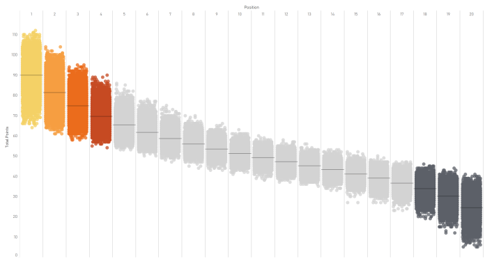
Let’s do this 10,000 times and look at the breakdown of points won by teams finishing in each position.

equal simulation 10k position x points.PNG

That’s a lot of variance! All of these teams are equal, and every single game had a 33.3% chance of the home team winning it, 33.3% chance of a draw, and 33.3% of the away team winning it. You’d think that this would balance out over the course of a season, but it doesn’t. A team can win the league with as many as 85 points (Random Athletic in simulation number 4349), a team can win the league with only 55 points (also Random Athletic, in simulation number 9384), a team can finish bottom with as many as 45 points (Real Random x2, Sporting Random, Random Argyle), and a team can finish bottom with only 18 points (Dynamo Random, Random United).

And if this is the amount of variance you can get between seasons when everything is equal, what happens when it’s not? Did West Ham get a particularly unlucky roll of the die when they finished 18th with 42 points, and that 36 points is going to see you to safety most of the time? Or is it that the last twenty or so seasons have been at the low end of the variance, and that in any given season, 36 points is still probably going to get you relegated? And is there even a points total where you’re definitely absolutely guaranteed not to get relegated?

On that last point, it’s technically possible to get relegated with 63 points. If two teams are completely useless and lose every single game, and the other 18 teams win every home game and lose every away game apart from the two games away to the bottom two, that means that 18 teams finish on 63 points (57 points from winning all home games, 6 points from winning two away games). One team could finish 18th on goal difference. So, really, 64 points is the real magic safety number.

But this would never realistically happen. So, I’ve also run 10,000 simulations of leagues based on real data. I took every single game from the last four years (2014/15 to 2018/19) of the big five leagues (England, Spain, France, Italy, Germany). Assuming that a team’s actual points total is a relatively good measure of a team’s actual strength – which it isn’t, as shown above, but it’s about as close as I can get – I drew random samples of 20 values for each simulation. Since Italy and Germany only have 18 teams in their top flights, I used each team’s average points per game (PPG) as their underlying team strength. This generated 10,000 realistic leagues of 20 teams of different strengths. I then grouped them into strength tiles of 0.3 points per game – the teams in the weakest tile were between 0.3 and 0.6 PPG, the teams in the strongest tile were between 2.4 and 2.7 PPG. I then compared the frequency of teams in each strength tile scoring a certain number of goals against teams in each strength tile, and sampled from those distributions for each of the 3,800,000 games in the simulations. I experimented with making the tiles smaller, but that meant that there were too few examples of games between teams of particular tiles. I also added a home vs. away boost factor.

This ended up coming out pretty realistic. For example, here’s the average number of goals that teams in each strength tile score and concede:

avg goals for and against per tile.PNG

So, what are the points distributions per position in a more realistic simulation?

accurate simulation 10k position x points.PNG

This looks pleasingly similar to the distributions in my graph of Premier League points by position. Most simulation results cluster around the middle of each band (the black line denotes the average). But at the extreme end, you can win the league with 112 points if you’re already a strong team and you outperform / get lucky, like Sporting Random did here:

highest winning total.png

…and you can also win the league with as little as 64 points if you outperform / get lucky and if the rest of the league underperform / get unlucky, like Real Random did here:

lowest winning total.png

At the bottom of the table, you can get relegated in 18th with 46 points, which is what happened to Random United, a solid midtable team who had a pretty average season… except that everybody else at the bottom of the table completely outperformed expectations / got incredibly lucky:

highest relegated total.png

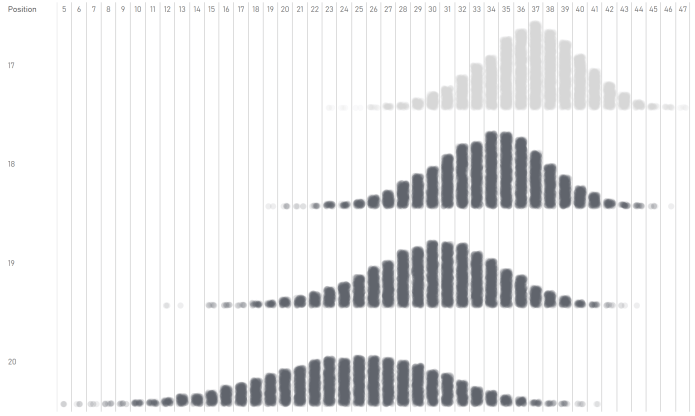
This chart shows the overlap between the relegation positions and safety. There are some interesting data points at the extreme ends, but the main point is that there are a lot of simulations where a team got 33 points or fewer but finished 17th, and there are several simulations where a team got 38 points or more but still finished 18th:

relegation points.PNG

To put it another way, 93% of teams getting 40 points didn’t get relegated:

cumulative percent curves

You can explore the full interaction between points and position in this graph, where you can set a threshold. Here, this shows how often a team finishes in a particular position when getting at least 40 points – so in 5.85% of simulations, you can get 40+ points, but still finish 18th:

% of teams per position

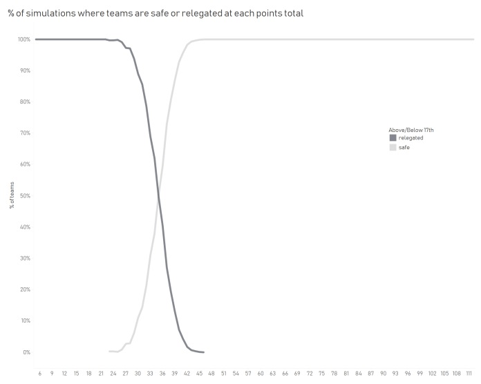
And to work out what your safety threshold is, this graph shows how many teams end up safe or relegated based on their points total. 35 is the turning point; 50.27% of teams getting 35 points end up safe:

% of relegations per points

As a final view, here’s a breakdown of the variance in positions by each team strength tile. It shows how you can be an incredibly strong team and expect to get 2.4 to 2.7 points per game, and you’ll win the league 63% of the time, but also miss out on the top four entirely a little under 1% of the time:

strength tiles and positions

Forty points isn’t a magic number – you’re safe around 93% of the time if you get 40 points, but it’s not guaranteed.

Standard
Alteryx, data visualisation, football, Tableau

The growing gap between the Premiership’s Top Six and the rest.

This is my first football data blog for a while, and I feel all nostalgic! It’s nice to dive into some league table data again, and even nicer now that I have Alteryx; I was able to format my data about 10x quicker than I was in when I first started doing this in R. Then again, I’ve probably also spent 5x more time using Alteryx than R in the last year or so. Anyway.

I’ve been hearing a lot more analysis of the Top 6 in the Premiership recently. I first noticed it in the last couple of seasons, when I saw a few journalists/people on Twitter writing about a “Big Six Mini-League”. Liverpool often seemed to do quite well at this, and Arsenal often seemed to do quite badly at this. Neither team won the actual league.

I’ve started looking at how the Top 6 sides in the Premiership perform each year (using data from this fantastically well-maintained repository), and there’s quite a few interesting stories in here. The first main point is that the big clubs are accelerating away from the rest of the league. The second main point is that any big six mini-league doesn’t really matter, as you can win the Premiership with an underwhelming record against your main rivals if you trash everybody else. I mean, that shouldn’t be much of a surprise – if you’re a Top 6 team, only 30 points are on offer from matches against your rivals, but you can potentially take 84 points from the 28 matches against the rest of the league.

For all these analyses, I’m taking Top 6 literally – meaning the teams that finish that season in the top six positions. Nothing to do with net spend, illustrious history, shirt sales in Indonesia, or anything like that. I then look at the average points-per-game changes by team, position, season, and Top 6/Bottom 14 status. I also filtered out the first three seasons of the Premiership to keep it slightly easier for comparison, since there were 22 teams in the league until 1995-96.

When plotting the average points-per-game per season between the two groups, a clear trend emerges; the Top 6 are better and better at beating the rest of the league:

1

However, this trend appears to be asymmetrical. When looking at the overall average points-per-game for all games across the season, teams that finish in the Top 6 are getting better, but there’s only a negligible decline for the rest of the league. This suggests the bigger, better teams are pulling away from the rest of the league:

2

This effect is most striking when plotting the difference in overall average points-per-game between the two groups:

3

Teams finishing in the Top 6 scored around 0.6 points-per-game more than the rest of the league in the early nineties, but that’s now up to over 1 point-per-game in the latest couple of seasons. That half-a-point difference translates to a 19-point difference across a whole 38-game season.

We can plot each team in each season of the Premiership (since 1995-96, when the league was first reduced to 20 teams) and look at how well they did against the top teams and the rest of the league. In this graph, the straight line represents equal performance vs the Top 6 and Bottom 14:

4

A couple of things stand out:

1. Only a handful of teams have ever done better vs. the Top 6 than the rest of the league. This seems to have no effect on final position.

2. It’s possible to win the league with a poor record against the Top 6 by consistently beating everybody else. Manchester United won the league in 00-01 and 08-09 with only 1.3 PPG vs the Top 6.

3. Manchester City this year are ridiculous.

I find it interesting to compare Liverpool and Arsenal over the years. One narrative I sometimes hear is that Liverpool tend to raise their game for big matches, but are too inconsistent the rest of the time, whereas Arsenal struggle against big sides but do well enough in the rest of the league to consistently finish well. This chart seems to bear that analysis out; Liverpool’s cluster of dots are higher on the chart, but further to the left:

6

…while Arsenal’s cluster is slightly lower but further to the right… and most importantly, more colourful:

5

And if you want to explore other teams and seasons, there’s an interactive version of all these graphs here.

Standard
Alteryx, football, Maps, Tableau

Centre of Gravity, Metaphorically: Plotting time-based changes on maps

I haven’t written a blog in far too long. My bad. So, to get back into the swing of things, here’s something I’ve been playing with this week: centre of gravity plots.

It started with an accident. I had some EU member data, and I was simply trying to make a filled map based on the year each country joined, just to see if it was worth plotting. You know, something like this:

1 eu filled.png

Except that I’d been having a clumsy day (the kind of day where I spilled coffee on my desk, twice), and accidentally missed the filled map option and clicked line instead:

2 broken line.png

Now, I normally don’t like connected scatterplots, but realised that I could change a couple of things to this accident to make quite a nice connected scatterplot on a map, joining up the central latitude and longitude of each country, so I thought I’d follow through with it and see what happened.

(by the way, the colour palette I use is the Viridis Palette, which I absolutely love. You can find the text to copy/paste into your Tableau preferences file here)

Firstly, I changed my “year joined” field from a discrete dimension into a continuous measure so that I could make it a continuous line with AVG(Year joined):

3 connected line left right.png

This connects all the countries by their central latitude and longitude as generated by Tableau, but it joins them up in order from left to right on the map. So, I then added AVG(Year joined) to the path shelf as well, which means that each country is joined in chronological order, or in alphabetical order when there’s a tie (as with Belgium, France, Germany, Italy, Luxembourg, and the Netherlands, who formed the EU in 1958):

4 connected line year.png

I was pretty happy with this; it shows the EU’s expansion eastwards over time far, far better than the filled map did.

I got talking to Mark and Neil online, who introduced me to the idea of “centre of gravity” plots, which show the average latitude and longitude of something and how it changes with respect to something else (usually time). In this case, a centre of gravity plot of the EU would show the average central point of Belgium, France, Germany, Italy, Luxembourg, and the Netherlands in 1958, then the average central point of Belgium, France, Germany, Italy, Luxembourg, the Netherlands, Denmark, Ireland, and the UK in 1973… and so on. I figured it should be easy enough, I’d just take Country off detail, replace it with Year joined, and average the latitudes and longitudes together.

Sadly, it doesn’t work that way. The Latitude (generated) and Longitude (generated) fields that Tableau automatically generates when it detects a geographic field like country can’t be aggregated, and can’t be used if the geographic field they’re based on isn’t in the view. That meant I couldn’t average the latitudes and longitudes over multiple countries without creating lots of different groups.

But, there’s a simple way around this! You can create a text table of the latlongs, copy/paste them into Excel or whatever, then read that in as another data source. Firstly, drag your geographic field into the view, and put the latitude on text, like so:

5 create table.png

Then copy and paste it all (I just click on there randomly, hit ctrl+A, ctrl+C, switch to Excel, ctrl-V). Now do the same for the longitude. Save the document, and read it in as a separate data source in Tableau. Now you can blend the data on Country, or whatever your geographic field is, and you’ve got actual latlongs that you can use like proper measures.

And so I did. I recreated the line chart with the new fields, but took Country off detail, and made AVG(Latitude) and AVG(Longitude) into moving average table calculations which take the current value and an arbitrarily high number of previous values (I put in 100, just because). This looked pretty good:

6 cog flawed averages.png

…but then I realised that it wasn’t accurate data. Look at the point for 1973, after the UK, Ireland, and Denmark joined. Doesn’t that seem a little far north?

7 cog flawed illustrated

To investigate it fully, I duplicated the sheet as a crosstab, because sometimes, tables are the best way to go. What I found is that I’ve got a bit of Simpson’s Paradox going on; the calculation is taking averages of averages:

8 cog flawed explained.png

Not so great. If we add Country to the view after the Year joined pill, you can see what it should be:

9 what it should be doing.png

But the problem is, how do we put Country on detail but then get the moving average to ignore it? I tried various LODs, but couldn’t get it to work exactly – if you have a solution, I would love to hear it! My default approach is to try to restructure the data in Alteryx – because that generally solves everything – but I feel like I’m becoming too reliant on restructuring the data rather than working with what Tableau can do.

Anyway, I ended up restructuring the data by generating a row for each country and year that the country has been a member of the EU. That means I can create a data table like this:

10 restructured table

…which removes the need for a moving average calculation entirely, because the entire data is moving with the year instead. Just take country off detail / out of the view, and you get the right averages:

11 restructured table 2

Much more accurate:

12 EU cog.png

This is a better way of structuring the data for this particular instance, because the dataset is tiny; 28 countries, 60-ish years, 913 rows in my Excel file. It’s not going to be a good, sustainable solution for a centre of gravity plot over a much bigger dataset though. I did the same thing for the UN – 193 countries, 70-ish years – and ended up with 10,045 rows in my Excel file. It’s easy to see how this could explode with much more data.

It does look interesting, though; I’d never have guessed that the UN’s centre of gravity hadn’t really left the Sahara since its inception:

12 UN cog

Finally, since I was on a roll, I plotted the centre of gravity for the English football champions since the first ever professional season in 1888-89. Conceptually, this was slightly different; unlike the EU and the UN, the champion isn’t a group of teams constantly joining over the years (although it is possible to plot that too). Rather, I wanted to create a rolling average of the centre of gravity over the last N years. If you set it to five years, it’s a bit messy, moving around the country quite a lot:

13 english football 5 years.png

But if you set it to 20 years, the line tells a nice story. You can see how English football started out with the original northern teams being the most powerful, then it moves south after the Second World War, then it moves north-west during the Liverpool/Manchester era of domination, and finally it’s moving south again more recently:

14 english football 20 years.png

Many thanks to Ian, who showed me how to parameterise this. Firstly, put your hard-coded (i.e. not Tableau generated!) latitude or longitude field in the view, and create a moving average over the last ten years. Or two, or thirteen, or ninety-eight, it doesn’t really matter. Next, drag the moving average latitude/longitude pill from the rows/columns into the measures pane in order to store it. This creates a calculated field. Meanwhile, create a parameter to let you select a number. This will change the period to calculate the moving average over. Open up the new calculated fields, and replace the number ten/two/thirteen/ninety-eight with your newly-created parameter, remembering to leave the minus sign in front of it:

15 calc mov avg param

This will let you parameterise your moving average centre of gravity.

It was a lot of fun to play around with these maps this week. I’ve packaged them all up in a Tableau Public workbook here; I hope you find it as interesting as I did!

(title inspiration: Touché Amoré – Gravity, Metaphorically)

Standard
Alteryx, football, Tableau

The relationship between away team performance and distance travelled in the English football league

If you follow football, you often hear about arduous away trips to the other side of the country. This seems to imply that the further an away trip is, the more difficult it is for the away team.

However, is that actually true? Do away teams really do worse when they’ve travelled a long way to get there, or is there no difference?

The football league season has just finished, so I’ve taken each match result from the Championship, League One, and League Two in the 2016-17 season. After some searching, I got the coordinates of each football league team’s stadium, and used the spatial tools in Alteryx to calculate the distance between each stadium. I then joined that to a dataset of the match results, and you can download and play with that dataset here. I stuck that into Tableau, and you can explore the interactive version here.

First, let’s have a look at how many points away teams win on average when travelling different distances. I’ve broken the distance travelled into bins of 25 miles as the crow flies from the away team’s stadium to the home team’s stadium, then found the average number of points an away team wins when travelling distances in that bin (I excluded the games where the away team travelled over 300 miles as there were only two match ups in that bin – Plymouth vs Hartlepool and Plymouth vs Carlisle).

It turns out that it actually seems easier for away teams when they travel further away:

Teams travelling under 25 miles win just under a point on average, while teams travelling over 200 miles win between 1.3 and 1.6 points on average.

This is surprising, but there could be several reasons contributing to this:

  1. Local rivalries. It’s possible that away teams do worse in derby matches than in other matches; this is something to investigate further.
  2. Team bonding. It’s possible that travelling a longer distance together is a shared experience that can help with team bonding.
  3. Southern economic dominance. England is relatively centralised, economically speaking; most of the wealth is in the south. Teams in the South travel further than average to away games, so perhaps the distance advantage actually shows a southern economic advantage; teams in richer areas can buy better players.
  4. Centralisation vs. sparser regions. England is relatively centralised, geographically speaking; most of the population lives in the bits in the middle, and teams in the Midlands travel the least distance on average. Perhaps teams in more centralised areas (e.g. Walsall, Coventry) have more competition for resources like new talent and crowd attendance, while teams in less centralised areas (e.g Exeter, Newcastle) might have less competition for those resources.

I also used Tableau’s clustering algorithm to separate out teams and their away performances based on distance travelled, and it resulted in four basic away performance phenotypes (which you can explore properly and search for your own team here):

Since I had the stadium details, I had a look at whether the stadium capacity made a difference. This isn’t a sophisticated analysis – better teams tend to be more financially successful and therefore invest in bigger stadiums, so it’s probably just a proxy for how good the home team is overall, rather than capturing how a large home crowd could intimidate an away team.

Finally, this heat map combines the two previous graphs and shows that away teams tend to do better when they travel further to a smaller ground. This potentially shows the centralisation issue discussed earlier; the lack of data in the bottom right corner of the graph shows that there are very few big stadiums in parts of the country like the far North West, North East, and South West, where away teams have to travel a long way to get to.

So, it looks like the further an away team travels, the better they tend to do… although that could reflect more complicated economic and geographic factors.

Standard